Bisection Method Using MATLAB

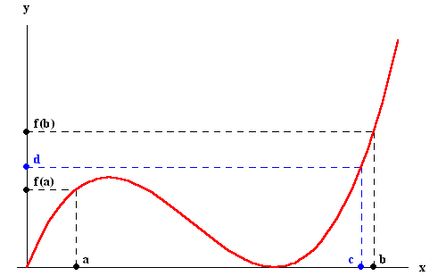
Bisection method is based on Intermediate Value Theorem which states as,
 Let f (x) be a continuous function on the interval [a, b]. If d  [f (a), f (b)], then there is a c  [a, b] such that f (c) = d.

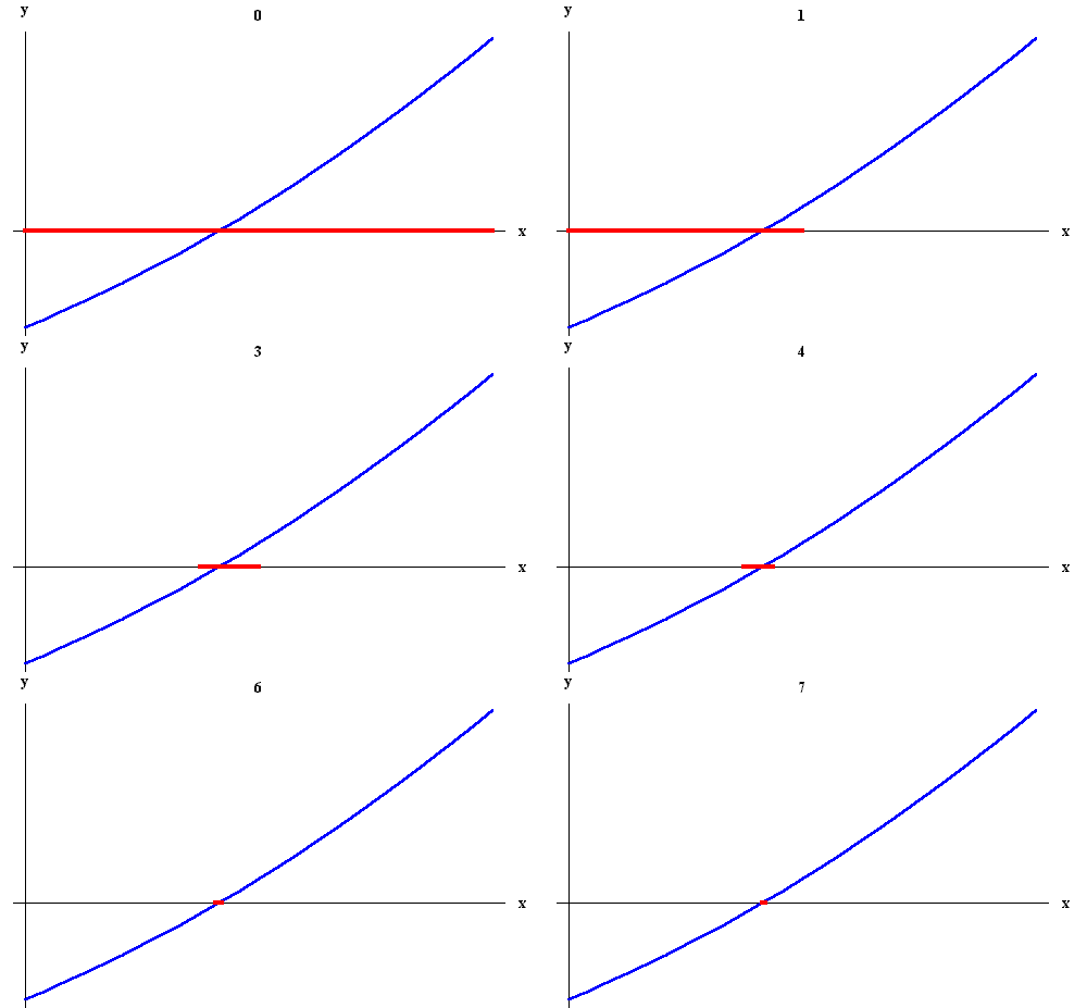
We are using a sub-form  form of this theorem, In our case we are given with two values at which function changes its value form positive to negative and we have to find a value where function is zero or in other words root of the function. We then use a binary search type algorithm that slowly decreases this interval and finally gets solution with some error. 

So if we are given with a interval [xl , xu] as lower and upper limit. Value of function with xl is negative and with  xu is positive then there must be at least one point in between these two values which is  root of the function  or in other words function becomes zero. Function should be real and continuous.

Algorithm:

1. We check weather function changes its value from positive to negative within given interval, If it changes we proceed other wise we can't find solution.
2. We find mid point of the interval, xm. 
3. If function at  xm is negative, it becomes our new xl, if its positive its our new xu and if it happens to be zero, we find our root (It rarely happens). 
4. We find error by seeing the difference between last and new xm. If error is smaller than provided one, we stops other wise step 2 and 3 repeats.
5. If we also limit iterations by 1000. Means our program can execute more than 1000 iterations.

MATLAB Code:

%Author: Muhammad Awais
%UET Lahore, Electrical Engineering
%fb/awais12506
function [iteration,xm]=Bisection(xl,xu,f,e)

%Find Root of a equation by method of BiSection
%Input: Lower Limit, Upper Limit, Function, Error Tolerance
%Please Insert f as f=@(x)x.^2+9*x+3
%Output: Root of the equation with given precison
%Exception: Give error if Equation is not convergent or roots are dont give

%postive and negative values of the function

iteration=0;     %To see how many iterations, equation took to solve
xm=xl;
error=1;
if  (f(xl)*f(xu)>0)
    disp('Interval have some error')

else
     while ( abs(error) > abs(e) ||iteration<=1000 )
        iteration=iteration+1;
        xmOld=xm;
        xm=(xl+xu)/2;   %Mid point
        xmNew=xm;
        if f(xl)*f(xm)<0   %if f(xm) is neg, equate xu with xm
            xu=xm;
        else if f(xl)*f(xm)>0 %if f(xm) is pos, equate xl with xm
            xl=xm;
            else            %it means xm is our root
            break
            end
        error=(xmNew-xmOld)/xmNew;   %Error
        end

    end

end
end

Output:

References:

http://www.sosmath.com/calculus/limcon/limcon07/limcon07.html

YBus building algorithm of Power System using MATLAB

Nodal admittance matrix or Ybus matrix is a matrix that contains admittances of the power system. This matrix can be used to find voltages of buses.

This Ybus matrix can be found easily and then inverted and multiplied with currents to find voltages of buses. Although taking inverse of a large system is computationally not efficient and there are ways to find Zbus directly instead of taking inverse of Ybus.

Ybus is sparse matrix with a lot of zeroes in it. So its a large matrix with a lot of zeroes.

Algorithm used in our code is  of 3 steps.

1.     Circuit is converted into matrix from called data. First column of data contains from and second contains to means nodes to which a admittance is connected. Third and forth contains value of resistance and reactance respectively.

2.     Off-diagonal entries are just net admittances connected to node i and j.

3.     Diagonal entries contains sum of all entries connected to that node. For example Y 3,3 is net of all the entries connected to bus 3.

Code:

%Author: Muhammad Awais

%Electrical Engineering, UET Lahore

%Bus admittance matrix

%Write buss impedence in Z matrix and it will solve rest of the thing

%data matrix

   data=[0   1   0   1j

   0   2   0 0.8j

   1   2   0 0.4j

   1   3   0 0.2j

   2   3   0 0.2j

   3   4   0 0.08j];

 % from  to R   X

%Z=[0   1   0   1j

 %  0   2   0 0.8j

 %  1   2   0 0.4j

  % 1   3   0 0.2j

   %2   3   0 0.2j

   %3   4   0 0.08j];

%finding order of matrix in C language way

%o1=max(Z(:,1));

%o2=max(Z(:,2));

%order=(max(o1,o2))

%find number of rows of Z= Toatl number of nodes

%row=length(Z(:,1))

[row,col]=size(data);

order=col

%Change last column into admittance, now last column also inculdes R

for m=1:row

    data(m,4)=1/(data(m,3)+data(m,4));

end

Z2adm=data;

%Yadmittance as a matrixo of zeros first

Y=zeros(order,order);

%finding ybus matrix

%1-for off-digonal vlaues

for i=1:row

    for j=1:order

        %discard source node

        if data(i,1)==0||data(i,2)==0    

           a=0;

         %for off digonal entries

        elseif data(i,1)~=0||data(i,2)~=0

            Y(data(i,1),data(i,2))=-data(i,4);

            Y(data(i,2),data(i,1))=-data(i,4);

        end

        

    end

end

%2-digonal values 

for a=1:order     %for k

    for b=1:row

        if data(b,1)==a ||data(b,2)==a

           

            Y(a,a)=(Y(a,a)+data(b,4));

        end

    end

   

end

Ybus=Y

%To find Z bus

Zbus=inv(Y)

%As Ibus=Ybus*Vbus so we can find too if we know Ibus. As here two currnet

%sources so suppose

Ibus=[1;1;0;0];

Vbus=Ybus\Ibus

Examples:

Example 1: To solve following system using this method

Impedance Matrix:

data=[0   1   0   1j

   0   2   0 0.8j

   1   2   0 0.4j

   1   3   0 0.2j

   2   3   0 0.2j

   3   4   0 0.08j];

Results:

Ybus =

        0 - 8.5000i        0 + 2.5000i        0 + 5.0000i        0         

        0 + 2.5000i        0 - 8.7500i        0 + 5.0000i        0         

        0 + 5.0000i        0 + 5.0000i        0 -22.5000i        0 +12.5000i

        0                  0                  0 +12.5000i        0 -12.5000i

Zbus =

        0 + 0.5000i        0 + 0.4000i        0 + 0.4500i        0 + 0.4500i

        0 + 0.4000i        0 + 0.4800i        0 + 0.4400i        0 + 0.4400i

        0 + 0.4500i        0 + 0.4400i        0 + 0.5450i        0 + 0.5450i

        0 + 0.4500i        0 + 0.4400i        0 + 0.5450i        0 + 0.6250i

Vbus =

        0 + 0.9000i

        0 + 0.8800i

        0 + 0.8900i

        0 + 0.8900i

Example 2:

Impedance Matrix:

data=[0   1   0  0.25j

   0   1   0  -4j

   1   4   0   0.4j

   1   3   0   .1j

   0   2   0    .2j

   0   2   0    -4j

   0   3   0    -4j

   0   3   0.9412  .2353j

   3   4   0      0.2j

   0   4   0     -4j

   0   4   .4706  0.11765j

    ];

Results:

Ybus =

        0 -20.2500i        0 + 4.0000i        0 +10.0000i        0 + 2.5000i

        0 + 4.0000i        0 -15.0000i        0                  0 + 6.2500i

        0 +10.0000i        0             1.0000 -15.0000i        0 + 5.0000i

        0 + 2.5000i        0 + 6.2500i        0 + 5.0000i   2.0000 -13.9998i

Zbus =

   0.0359 + 0.1305i   0.0303 + 0.0718i   0.0481 + 0.1134i   0.0498 + 0.0887i

   0.0303 + 0.0718i   0.0264 + 0.1224i   0.0398 + 0.0744i   0.0439 + 0.0878i

   0.0481 + 0.1134i   0.0398 + 0.0744i   0.0652 + 0.1733i   0.0648 + 0.1061i

   0.0498 + 0.0887i   0.0439 + 0.0878i   0.0648 + 0.1061i   0.0736 + 0.1538i

Vbus =

   0.0662 + 0.2023i

   0.0567 + 0.1941i

   0.0879 + 0.1878i

   0.0937 + 0.1765i

Reference:

Examples were taken from Power System Analysis - Hadi Saadat